Testing out integrating plotly.js charts into the blog by going straight making animations of systems of differential equation to test their performance. The article image is, of course, not actually interactive, and the article read time is accurate only if you read the page source of the plots.
Plots
Suppose now that I’ve edited this site to support plotly, I should produce some content with them and have chosen to go with some applied math classics. Plotly is pretty easy to use, but the documentation and examples for making figures via their python library are poor.
Lotka-Volterra ODE system
The Lotka-Volterra model is one of the simplest predator-prey dynamics models demonstrating stable limit cycles, meaning the system enters a fixed oscillatory pattern. It consists of a population of prey $x(t)$ that grows exponentially with growth rate $\alpha$, a predator population $y(t)$ that starves exponentially with death rate $\gamma$, and interaction terms of predation causing the growth of the predators and deaths of the prey proportional to the product of their populations (more hungry predators eat more available prey). This system is defined as:
$$ \frac{dx}{dt} = \alpha x - \beta xy ,$$ $$ \frac{dy}{dt} = \delta xy - \gamma y ,$$
where $\alpha, \beta, \delta, \gamma > 0$. The chart that follows is of the Lotka-Volterra system with $\alpha = 2/3$, $\beta=4/3$, $\gamma=1$, $\beta=1$, and integrated numerically from $t=0$ to $t=20$ with step size $\Delta t=0.04$, with a few different initial conditions. Small dots represent the initial position at $t=0$, and large dots $x(t)$, $y(t)$. The trajectory over time is shown as lines in the same color.
We see here from integrating these equations gives a boom-bust cycle in the populations of predator and prey. I’ll leave you to guess or what initial point with these conditions is an equilibrium point.
This system of ODEs is also a bit unusual in that it gives rise to a family of limit cycles, as we can see each initial condition we have plotted defines an orbit that does not intersect the others. This unusual behavior arises in that these equations happen to have a conserved quantity $f(x(t),y(t))=V$ for all $t$. In the next example we will look at the van der Pol oscillator, a system with a stable limit cycle that attracts trajectories from different initial values.
Van der Pol Oscillator
A common example of a system possessing a stable limit cycle is one studied in the early 1900s by Balthazar van der Pol, an early researcher of analog electronic circuits. Similar oscillators describe dynamics of pendulums, or more complicated signals such as heart rhythms or neuron action potentials.
What circuit this particular equation comes from is not wholly clear to me, but is generally given in applied mathematics texts as the following dimensionless second-order differential equation:
$$ \frac{d^2x}{dt^2} -\mu (1-x^2) \frac{dy}{dt} + x = 0. $$
This ODE is converted to a system of first order differential equations for numerical integration by letting $\frac{dx}{dt} = y$ and substituting, giving:
$$ \frac{dx}{dt} = y $$ $$ \frac{dy}{dt} = -x + \mu (1-x^2) y $$
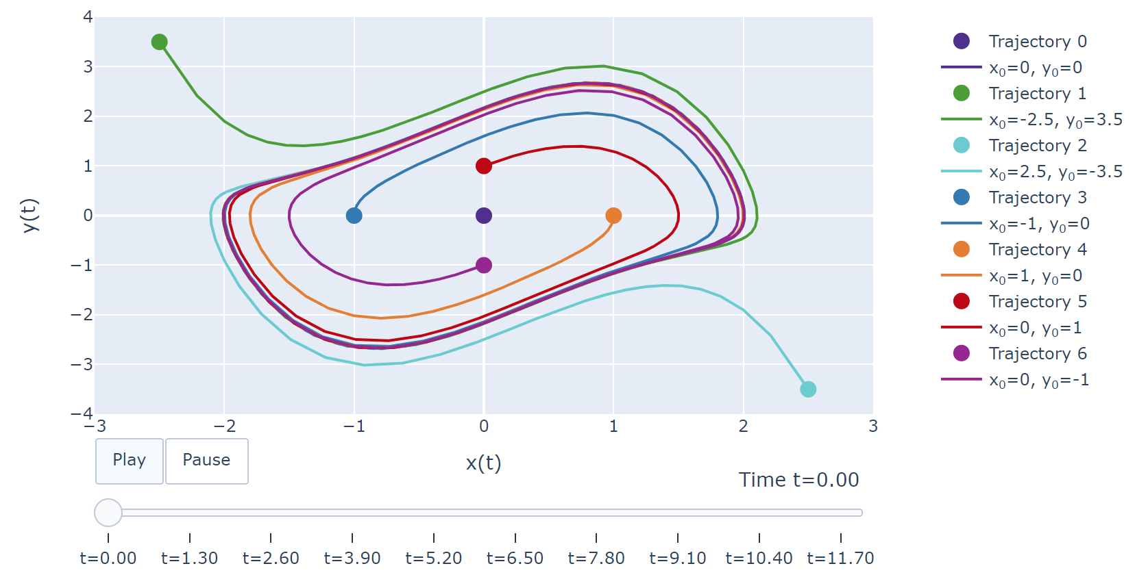
Setting $\mu=1$, we then integrate and plot the system for multiple initial conditions. See code links below if you want exact integrator settings.
The center (0,0) is an unstable fixed point, and we observe that trajectories near it move outwards towards the stable limit cycle, and that trajectories outside of the limit cycle are attracted towards it. Thus, this illustrates that this system’s limit cycle is stable.
For those interested into diving into this system further, a good lecture video by Steven Strogatz is online from Cornell. His book Nonlinear Dynamics and Chaos is a reasonable read and introduction to these topics as well.
Plot Code
The scripts to generate the embedded plots are in the Github repository I use to keep this blog, alongside this post.
The scripts are a bit of a mess, but are surely better than the current animation examples for making plotly animations in python. Will see if I find the time to submit pull requests to their documentation.
Reminders to self of future-content
Readers are welcome to badger me as well. I’ll probably get a post out soon on percolation, and I think a post discussing a system of equations that has hysteresis - maybe a model of forests, where the equilibrium conditions of the forest depend not only on the current conditions, but on the past history of the forest. I suppose other people would call this a “tipping-point”. Forthcoming hopefully, abandonware maybe.


